Speed

Tests show that standard cone bearings have less friction than sealed ball bearings

Traditional cup and cone bearings were compared with cartridge bearings with and without seals. Two types of lubricant were also compared. For each bearing configuration, measurements of the frictional drag torque were made for different types of bearings with loads varying between zero and 264 N and rotational speeds up to 600 rpm. For a typical road racing bike, this would correspond to a speed of 48 mph.

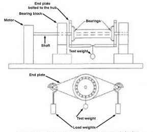
Test method

A shaft was driven by an electric motor. The shaft passed through large pillow block bearings supporting the assembly. A bicycle hub was mounted between the pillow block bearings with the shaft replacing the axle. At each end of the hub, a plate was attached. On either side of the hub, running parallel to the shaft, knife edges connected the plates to each other. Load weights were suspended between the knife edges. This arrangement allowed the load weights to apply a vertical force to the bearings while remaining balanced so as not to offer any moment resisting rotation of the hub. An additional test weight was suspended from the plates directly below the center of the bicycle hub. When the shaft is rotated, friction causes the hub to rotate. This rotation moves the test weight out of alignment with the shaft so that it produces a restoring moment. At equilibrium, the frictional moment is equal to the restoring moment and from the angle of the hub, the friction can be calculated.

To minimize the effects of inertia and friction within the knife-edge, the hub was disturbed so that it rocked. Measurements were taken after the resulting oscillations had damped out, as well as in both directions. These measurements were averaged.

Cartridge bearings were tested as supplied (with seals and factory fitted grease), with grease removed and replaced by 20 W oil, and with seals removed but original grease remaining. The cup and cone bearings were tested after careful setup to minimise friction, with both 20 W oil and with an automotive chasis grease.

Results

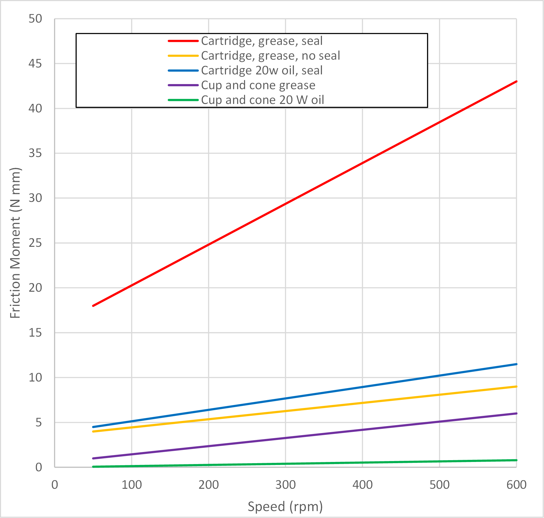
Surprisingly the results show that friction appears to be linearly dependent on rotational velocity but had no dependence on loading. The results also showed that sealed cartridge bearings had several times more friction when lubricated with grease than with oil. This was also true for cup and cone bearings. The effect of removing the seals from the sealed bearings was much more modest. Cup and cone bearings, lubricated with oil, had the lowest overall friction.

It is noted that the friction for bearing seals may be high as new bearings were used. Seals bed-in with use and their friction therefore reduces.

In the paper, charts are presented with straight lines fitted to the experimental data. The coefficients of these lines are not given although they would be the most useful way to present the findings. It would then be possible to represent the resulting resistance force as a function of these coefficients, the wheel radius and the velocity of the bicycle.

F_WB = C_WB0  / r   +   (C_WB1 * 1000  / r²) * v

Where C_WB0 and C_WB1 are the coefficients, r is the wheel radius (mm) and v is the ground velocity (m/s). The factor of 1000 is required since the wheel radius is given in mm but the velocity is in m/s. Interpreting the data given in the charts in this paper, the coefficients will take the following values:

Bearing type	CWB0	CWB1
Cartridge, grease, seal	15.7	0.434
Cartridge, grease, no seal	3.5	0.087
Cartridge 20w oil, seal	3.9	0.122
Cup and cone grease	0.5	0.087
Cup and cone 20 W oil	0.0	0.013

Reference:

Title: Frictional resistance in bicycle wheel bearings, Cycling Science
Authors: K Danh, L Mai, J Poland, C Jenkins
In: Cycling Science, 1991, Vol.3(3-4), p.28-32

Read the full paper…

Resistance parameters measured for real cyclists intercepted in Vancouver

For the first time, scientists have reliably measured how efficient typical urban bikes actually are. Their study showed that most people’s bikes are much slower than previously thought. There is also more variation between different bikes.

Two things primarily determine how fast a bike is when riding on level ground – the aerodynamic drag and the rolling resistance. Aerodynamic drag is represented by the effective frontal area while rolling resistance is represented by a dimensionless coefficient. Estimates for the values for these resistance parameters have previously focused on sport cyclists. Although some measurements have been made for urban utility bikes, these have been carried out under idealized conditions.

Method

In this study, scientists stopped real cyclists on a bike path in Vancouver and tested their bikes. The rolling resistance and aerodynamic drag were measured using a coast-down test. This involves the cyclist coasting from a cruising speed to a stop, while the speed of the bike is accurately measured. Since rolling resistance causes a constant force, while drag causes a force that depends on the velocity squared, it is possible to estimate both parameters by fitting a curve to the speed measurements.

Coast-down isn’t as accurate as other methods such as wind tunnel tests but it is convenient for cyclists that have been intercepted on their way past. For this study, infrared time traps were used to measure the speed of the cyclists as well as ultrasonic anemometer measurements to correct for wind speed. The test was rigorously evaluated and found to be sufficiently accurate. The uncertainty (standard deviation) of the coefficient of rolling resistance was 0.001 and for the effective frontal area, it was 0.1 m². The air density was estimated from altitude and temperature using the equation:

where ρ₀=1.293 kg/m³, h is altitude above sea level in km and T is absolute temperature (k)

557 cyclists were intercepted and tested at 9 locations in Vancouver. They were aged between 6 and 80 and riding a wide range of bikes. Most cyclists coasted with pedals parallel to the ground which probably reduced drag slightly. If they had pedalled backwards, this would have more accurately represented the typical drag when cycling. Since the bikes were tested as they were found, the rolling resistance may, in some cases, include rolling resistance.

Results

The study showed that resistance parameters are higher than previously thought. This means that real bikes are slower than the ones previously measured.

The study showed that resistance parameters are higher than previously thought. This means that real bikes are slower than the ones previously measured.

The mean coefficient of rolling resistance of was 0.0077 with a standard deviation of 0.0035, after removing variation explained by the measurement uncertainty. The distribution had a skewness of 0.47 and was best approximated by a Weibull distribution. The range of values, after correcting for measurement variation, was from 0.001 to 0.015.

The mean effective frontal area was 0.559 m² with a standard deviation of 0.14 m² after correcting for measurement variation. The distribution had a skewness of 0.58 and was best approximated by a Gamma distribution. The range of values, after correcting for measurement variation, was 0.28 to 0.83 m². Assuming a typical air density of 1.2 kg/m³, these results equate to dimensionless drag factors (KA), of between 0.17 and 0.5.

The mean combined mass of bicycle and cargo was 18.3 kg with a standard deviation of 4.1 kg.

Results showed the expected correlations with wider and more upright rider positions causing more aerodynamic drag, and lower pressure tires with larger treads causing more rolling resistance.

Abstract:

This study investigates the rolling and drag resistance parameters and bicycle and cargo masses of typical urban cyclists. These factors are important for modelling of cyclist speed, power and energy expenditure, with applications including exercise performance, health and safety assessments and transportation network analysis. However, representative values for diverse urban travellers have not been established. Resistance parameters were measured utilizing a field coast-down test for 557 intercepted cyclists in Vancouver, Canada. Masses were also measured, along with other bicycle attributes such as tire pressure and size. The average (standard deviation) of coefficient of rolling resistance, effective frontal area, bicycle plus cargo mass, and bicycle-only mass were 0.0077 (0.0036), 0.559 (0.170) m², 18.3 (4.1) kg, and 13.7 (3.3) kg, respectively. The range of measured values is wider and higher than suggested in existing literature, which focusses on sport cyclists. Significant correlations are identified between resistance parameters and rider and bicycle attributes, indicating higher resistance parameters for less sport-oriented cyclists. The findings of this study are important for appropriately characterising the full range of urban cyclists, including commuters and casual riders.

Reference:

Title: Physical characteristics and resistance parameters of typical urban cyclists
Authors: Simone Tengattini; Alexander York Bigazzi
ISSN: 0264-0414 , 1466-447X; DOI: 10.1080/02640414.2018.1458587
In: Journal of sports sciences, 2018, Vol.36(20), p.2383-2391

Read the full paper…

A full-scall wind tunnel test method has been created at RMIT University. The bicycle is mounted on a platform which is itself mounted on a load cell. The load cell has 6 degrees of freedom (DoF) allowing drag, lift and side forces to be measured. The bicycle can be orientated at different yaw angles to the airflow so that the effects of crosswind can be observed. However, non-zero yaw angles increase the frontal area beyond the recommended maximum of 10 percent  solid blockage ratio for the 6 m² RMIT wind tunnel. The platform measures 1,800 mm × 850 mm × 30 mm and is mounted just 20 mm from the tunnel floor to minimize interference. A plastic fairing is fitted to the front of the platform to further reduce flow separation. Video cameras are mounted around the cyclist to monitor any changes in body position.

Previous research has shown that aerodynamic drag causes the majority of resistance to a cyclist’s motion. For example, Kyle and Burke showed that for road bikes travelling on a level surface aerodynamics accounted for 50 percent of total drag at 13 kph (8 mph) increasing to 90 percent at 32 kph (20 mph). Other researchers have found the contribution to be just 50% at the higher end of this speed range for mountain bikes, perhaps because of considerably higher rolling resistance. Approximately 31-39 percent of the aerodynamic drag is caused by the bike with the rest caused by the rider and clothing.  The position of the rider has a significant impact on the drag.

Direct measurement of the drag force was used to determine the drag coefficient using the standard equation:

where F_D is the drag force, rho is the air density, V is the speed and A is the projected frontal area of the cyclist and bicycle. The frontal area was measured using a digital camera and image processing software. Experiments using this setup have shown standard deviations in the drag coefficient of less than one percent for a wide range of riding positions.

A major weakness of the approach documented in the paper is that the wheels of the bicycle are not rotated. The rotation of the wheels changes the flow of air and therefore affects the horizontal drag force. This is something considered by other researchers and yet not explaination for omitting it is given. There is also air resistance to the rotation its-self, something not considered by most studies.

Results

This study measured the frontal area and then calculated the coefficient of drag Cd for each riding position. It showed a very slight dependence of
Cd on velocity, which for most purposes could be ignored.

The following values were recorded:

	Cd at 20 kph	Cd at 70 kph	Area m2
Recreational rider in upright position	1.16	1.13	0.54
Professional cyclist on tops	1.04	1.02	0.411
Professional cyclist on drops	1.02	1	0.405
Professional cyclist on aero bars	0.87	0.88	0.38

Abstract:

Aerodynamically efficient sports equipment/accessories and athlete body postures are considered to be the fundamental aspect to achieve superior performance. Like other speed sports, the aerodynamic optimisation is more crucial in cycling. A standard full-scale testing methodology for the aerodynamic optimisation of a cyclist along with all accessories (e.g., bicycle, helmet, cycling suit, shoes and goggle) is not well developed, documented, and standardised. This paper describes a design and development of a full-scale testing methodology for the measurement of aerodynamic properties as a function of cyclist body positions along with various accessories over a range of wind speeds. The experimental findings indicate that the methodology can be used for aerodynamic optimisation of all cycling sports.

Reference:

Bicycle aerodynamics: an experimental evaluation methodology
Harun Chowdhury Firoz Alam
Sports engineering. , 2012, Vol.15(2), p.73-80
<a href=””>Read the full paper…</a>

Sophisticated model including slip and steering angles shows accuracy within 0.2 percent

This study sought to improve on the accuracy of existing models for the speed of a track cyclist. It was based on the governing equation:

where η is the transmission efficiency, P_in is the power delivered by the cyclist, dt is a discrete period of time, ΔT is the change in kinetic energy, ΔV is the change in potential engery and E_dis is the energy disipated by resistance forces.

The energy dissipation is calculated considering the usual resistance forces such as aerodynamic drag and rolling resistance. Significant improvements in accuracy were given by accounting for kinetic energy, including rotational, and varying rolling resistance due to cornering. This resulted in a high accuracy of predicted lap times with errors consistently less than 0.36 percent.

Abstract:

A review of existing mathematical models for velodrome cycling suggests that cyclists and cycling coaches could benefit from an improved simulation tool. A continuous mathematical model for cycling has been developed that includes calculated slip and steering angles and, therefore, allows for resulting variation in rolling resistance. The model focuses on aspects that are particular, but not unique, to velodrome cycling but could be used for any cycling event. Validation of the model is provided by power meter, wheel speed and timing data obtained from two different studies and eight different athletes. The model is shown to predict the lap by lap performance of six elite female athletes to an average accuracy of 0.36% and the finishing times of two elite athletes competing in a 3-km individual pursuit track cycling event to an average accuracy of 0.20%. Possible reasons for these errors are presented. The impact of speed on steering input is discussed as an example application of the model.

Reference:

A mathematical model for simulating cycling: applied to track cycling Fitton, B., Symons, D. 2018

Sports Engineering
21(4), pp. 409-418

Read the full paper…

Simplified method to calculate epicyclic transmission efficieny early in design

Standard methods for analyzing transmission efficiencies assume that all of the power flows through each gear in a sequence. In a hub gear, the planetary gear trains (PGTs) or epicyclic gear trains involve a number of planet gears transferring power in parallel. This requires special methods for efficiency analysis which are often time consuming to perform. This paper presents a simplified method. It has been validated against previously published results and may be useful for the evaluation of proposed designs.

The method in this paper only considers gear-mesh loses, caused by the sliding friction when the teeth mesh together, which normally provides a reasonably accurate calculation of efficiency. The procedure has the following steps:

1. List all fundamental circuits, consisting of two meshing geats and a carrier. For each, carry out kinematic analysis to solve for the angular speed of each link.
2. Find the idealized torque of each link, assuming there is no power loss.
3. Identify the direction in which power is flowing through each link
4. Add gear-mesh losses for each gear pair, giving the actual torque of each link
5. Sketch a power flow diagram and calculate the overall efficiency

The paper goes step-by-step through a method of calculating the efficiency of a hub gear system. If you want to perform the calculations you’ll need to read the full paper.

Abstract:

Purpose

The analysis of power flow and mechanical efficiency constitutes an important phase in the design and analysis of gear mechanisms. The aim of this paper is to present a systematic procedure for the determination of power flow and mechanical efficiency of epicyclic-type transmission mechanisms.

Design/methodology/approach

A novel epicyclic-type in-hub bicycle transmission, which is a split-power type transmission composed of two transmission units and one differential unit, and its clutching sequence table are introduced first. By using the concept of fundamental circuits, the procedure for calculating the angular speed of each link, the ideal torque and power flow of each link, the actual torque and power flow of each link determined by considering gear-mesh losses, and the mechanical efficiency of the transmission mechanism is proposed in a simple, straightforward manner. The mechanical efficiency analysis of epicyclic-type gear mechanisms is largely simplified to overcome tedious and complicated processes of traditionally methods.

Findings

An analysis of the mechanical efficiency of a four-speed automotive automatic transmission completed by Hsu and Huang is used as an example to illustrate the utility and validity of the proposed procedure. The power flow and mechanical efficiency of the presented 16-speed in-hub bicycle transmission are computed, and the power recirculation inside the transmission mechanism at each speed is detected based on the power flow diagram. When power recirculation occurs, the mechanical efficiency of the gear mechanism at the related speed reduces. The mechanical efficiency of this in-hub bicycle transmission is more than 96 percent for each speed. Such an in-hub bicycle transmission possesses reasonable kinematics and high mechanical efficiency and is therefore suitable for further embodiment design and detail design.

Originality/value

The proposed approach is suitable for the mechanical efficiency analysis of all kinds of complicated epicyclic-type transmissions with any number of degrees of freedom and facilitates a less-tedious process of determining mechanical efficiency. It is a useful tool for mechanical engineering designers to evaluate the efficiency performance of the gear mechanism before actually fabricating a prototype as well as measuring the numerical data. It also helps engineering designers to cautiously select feasible gear mechanisms to avoid those configurations with power recirculation in the preliminary design stage which may significantly reduce the time for developing novel in-hub bicycle transmissions.

Reference:

Computing the power flow and mechanical efficiency of in-hub bicycle transmissions

Wu, Yi-Chang; Cheng, Chia-Ho, 2014

In: Engineering Computations (Swansea, Wales) v 31, n 2

Read the full paper…

Many elite cyclists use wind tunnels to improve their aerodynamic performance. The wind tunnel gives information on the total drag in different positions. They can, therefore, try different positions to see which gives the lowest drag. This is something of a trial and error process. In this study Computational Fluid Dynamics (CFD) is used to simulate airflow and understand what is causing drag. This may allow design for better aerodynamic performance. The drag caused by each body part is calculated and the heat transfer coefficient is also calculated.

The analysis was carried out for three positions, the upright position, riding on the dropped handlebars and in a time trial position. For each position, a laser scanner was used to measure the cyclist, the bicycle was not modeled. Validation of the simulation model was carried out by comparison with full-scale wind tunnel experiments in which surface pressure was measured at 115 positions on the cyclist’s body.

19 body sections were considered. These were the head, neck, each arm, each side of the body, the chest, the back, 3 sections of the pelvis, the upper and lower section of each leg and each hand and foot. The head was the largest single contributor to drag in all positions.

Abstract:

This study aims at investigating drag and convective heat transfer for cyclists at a high spatial resolution. Such an increased spatial resolution, when combined with flow-field data, can increase insight in drag reduction mechanisms and in the thermo-physiological response of cyclists related to heat stress and hygrothermal performance of clothing. Computational fluid dynamics (steady Reynolds-averaged Navier-Stokes) is used to evaluate the drag and convective heat transfer of 19 body segments of a cyclist for three different cyclist positions. The influence of wind speed on the drag is analysed, indicating a pronounced Reynolds number dependency on the drag, where more streamlined positions show a dependency up to higher Reynolds numbers. The drag and convective heat transfer coefficient (CHTC) of the body segments and the entire cyclist are compared for all positions at racing speeds, showing high drag values for the head, legs and arms and high CHTCs for the legs, arms, hands and feet. The drag areas of individual body segments differ markedly for different cyclist positions whereas the convective heat losses of the body segments are found to be less sensitive to the position. CHTC-wind speed correlations are derived, in which the power-law exponent does not differ significantly for the individual body segments for all positions, where an average value of 0.84 is found. Similar CFD studies can be performed to assess drag and CHTCs at a higher spatial resolution for applications in other sport disciplines, bicycle equipment design or to assess convective moisture transfer.

Reference:

“Computational fluid dynamics analysis of drag and convective heat transfer of individual body segments for different cyclist positions”
Thijs Defraeye Bert Blocken Erwin Koninckx Peter Hespel Jan Carmeliet
Journal of biomechanics. , 2011, Vol.44(9), p.1695-1701

Read the full paper…

Validation of a Mathematical Model for Road Cycling Power

This important study was carried out to test whether existing mathematical models can accurately predict power during road cycling. It showed that the model can predict power with an accuracy of about 3 percent (standard error of 1.6 percent)

A number of resistance forces cause power consumption while a bicycle is in motion. These include aerodynamic drag, rolling resistance, friction in bearings, transmission losses, changes in potential energy and acceleration. Each of these resistance forces can be calculated based on experimentally determined constants, the combined mass of the bike and rider, the velocity of the bicycle, and environmental measurements. The resistance force, multiplied by the velocity, gives the power loss due to each factor. Using such an approach it is possible to predict how much power a cyclist requires to achieve a given speed.

Prior to this study, no tests had every actually measured the power produced by a cyclist during normal road cycling, together with the speed achieved. Such a comparison enables verification of the power calculation equation. The main reason was that power meters were not available. This study utilized an early commercial power meter, the SRM Training System.

Validation of Power Meter

The SRM power meter was compared with a cycle ergometer. This uses a frictiion belt passed over a drum, which moves a pendulum, to measure torque when cycling. It can be calibrated by hanging weights from the belt. Combined with measurement of cadence (speed of pedal-crank rotation) the power can be accurately measured.

The power measured by the SRM was found to be 97.698 percent of the power delivered to the ergometer. It was assumed that the SRM power was valid and that the chain drive efficiency was 97.698 percent. This was justified on the basis that this was the expected efficiency based on previous studies.

Determining parameters for mathematical model

The mathematical model included terms for:

• Aerodynamic resistance to forward motion
• Aerodynamic resistance to wheel rotation
• Rolling resistance
• Frictional losses in wheel bearings
• Changes in potential energy (slope resistance)
• Changes in kinetic energy (acceleration forces)
• Frictional loss in drive chain

Aerodynamic resistance to forward motion was calculated in the normal way, using the equation: F_A = ½ ρ C_d A v_A² .
ρ is the air density and v_A is the velocity of the air relative to the bike. The drag area (C_DA) was determined by measuring the drag force, air velocity and air density in the Texas A&M wind tunnel. Subjects pedaled at approximately 90 RPM and an electric motor was used to rotate the front wheel. This was done at a range of yaw angles to enable the drag area in any cross-wind conditions to be determined.

The aerodynamic resistance to wheel rotation was determined by using the SRM crank to rotate the wheels with the bicycle suspended above the ground. This gave the combined power to rotate the wheel, the bearings, and the chain. Independent measurements were made for rotating the hub with no wheel to determine how much of this was due to the bearings and chain. Since the wheel rotation resistance was assumed to be due to aerodynamic resistance, the resistance force was modeled as: F_WR = ½ ρ F_W v_A². The actual form of this equation was in terms of power but for consistency with other calculations on this site, the force form is used here. The factor F_W is used in place of C_DA to represent the incremental drag area of the spokes or disk. The rear wheel was a lens-shaped disk and the front wheel had an airfoil section rim with 24 oval spokes.

Note: Although this general approach is valid, it is incorrect to use the air velocity for wheel rotation. The speed of wheel rotation is related to the ground velocity, not the air velocity.

Rolling resistance was calculated in the normal way, as a ratio of the tangential force to the normal force. It was assumed that the rolling resistance factor C_R did not vary with velocity. No assumption was made for small angles of slope. The angle of slope was therefore found from the arctangent of the gradient. The normal force is then the cosine of this angle multiplied by the combined weight of bike and rider (mg). Tires of 20 mm width were used, inflated to 9 atmospheres (130 psi). Rolling resistance was not measured, average values from previous studies were used.

The frictional losses in wheel bearings were not assumed to be constant with velocity, citing Dahn. Mai, Poland, and Jenkins (1991).

Note: Confusingly, they state that bearing friction was shown to be dependent on both load and rotational speed, but then go on to present an expression for bearing torque which is only a function of the rotational velocity.

The torque in each bearing pair was given by: T = 0.015 + 0.00005N. where N is the rotational velocity in RPM. This gives the total resistance force as P_WG = 91 + 8.7v_G

Changes in potential energy were found by multiplying the slope resistance, calculated in the normal way, by the distance traveled to give the work done.

Changes in kinetic energy were also calculated using standard equations for constant acceleration. The difference in kinetic energy between the beginning and end of each trial was recorded.

Experimental Validation

Subjects rode along a straight 470 m length of concrete. The accelerated to a steady speed before entering the test section and decelerated after leaving it. Trails were carried out in both directions and at 4 different speeds varrying between 7 ma and 12 m/s (15 and 27 mph).

Powers measured by the SRM had a mean of 172.8 W with a range of 29.4 W. The powers predicted by the model had a mean of 172.0 W with a range of 30.4 W. The results were highly correlated with a standard error of 2.7 W. About 1.6%.

Abstract:

This investigation sought to determine if cycling power could be accurately modeled. A mathematical model of cycling power was derived, and values for each model parameter were determined. A bicycle-mounted power measurement system was validated by comparison with a laboratory ergometer. Power was measured during road cycling, and the measured values were compared with the values predicted by the model. The measured values for power were highly correlated (R² = .97) with, and were not different than, the modeled values. The standard error between the modeled and measured power (2.7 W) was very small. The model was also used to estimate the effects of changes in several model parameters on cycling velocity. Over the range of parameter values evaluated, velocity varied linearly (R² > .99). The results demonstrated that cycling power can be accurately predicted by a mathematical model.

Reference:

Validation of a mathematical model for road cycling power

Martin, James C. (Motor Control Laboratory, Department of Kinesiology, University of Texas at Austin); Milliken, Douglas L.; Cobb, John E.; McFadden, Kevin L.; Coggan, Andrew R.

In: Journal of Applied Biomechanics, v 14, n 3, p 276-291, Aug 1998

Read the full paper…